Gravitational Field and Gravitational Potential

TL;DR

• Newton’s law of universal gravitation: $\mathbf{F} = -G\cfrac{mM}{r^2}\mathbf{e}_r$
• For objects with continuous mass distribution and finite size: $\mathbf{F} = -Gm\int_V \cfrac{dM}{r^2}\mathbf{e}_r = -Gm\int_V \cfrac{\rho(\mathbf{r^\prime})\mathbf{e}_r}{r^2} dv^{\prime}$
  • $\rho(\mathbf{r^{\prime}})$: mass density at a point located at position vector $\mathbf{r^{\prime}}$ from an arbitrary origin
  • $dv^{\prime}$: volume element at a point located at position vector $\mathbf{r^{\prime}}$ from an arbitrary origin
• Gravitational field vector:
  • A vector representing the force per unit mass experienced by a particle in the field created by an object of mass $M$
  • $\mathbf{g} = \cfrac{\mathbf{F}}{m} = - G \cfrac{M}{r^2}\mathbf{e}_r = - G \int_V \cfrac{\rho(\mathbf{r^\prime})\mathbf{e}_r}{r^2}dv^\prime$
  • Has dimensions of force per unit mass or acceleration
• Gravitational potential:
  • $\mathbf{g} \equiv -\nabla \Phi$
  • Has dimensions of (force per unit mass) × (distance) or energy per unit mass
  • $\Phi = -G\cfrac{M}{r}$
  • Only the relative difference in gravitational potential has meaning; the specific value itself is meaningless
  • Usually the condition $\Phi \to 0$ as $r \to \infty$ is arbitrarily set to remove ambiguity
  • $U = m\Phi, \quad \mathbf{F} = -\nabla U$
• Gravitational potential inside and outside a spherical shell (Shell theorem)
  • When $R>a$:
    • $\Phi(R>a) = -\cfrac{GM}{R}$
    • When calculating the gravitational potential at any external point due to a spherically symmetric mass distribution, the object can be treated as a point mass
  • When $R<b$:
    • $\Phi(R<b) = -2\pi\rho G(a^2 - b^2)$
    • Inside a spherically symmetric mass shell, the gravitational potential is constant regardless of position, and the gravitational force is $0$
  • When $b<R<a$: $\Phi(b<R<a) = -4\pi\rho G \left( \cfrac{a^2}{2} - \cfrac{b^3}{3R} - \cfrac{R^2}{6} \right)$

Gravitational Field

Newton’s Law of Universal Gravitation

Newton had already systematized and numerically verified the law of universal gravitation before 11666 HE. Nevertheless, it took another 20 years until he published his results in his book Principia in 11687 HE, because he could not justify the calculation method that assumed the Earth and Moon as point masses without size. Fortunately, using the calculus that Newton himself invented later, we can prove that problem, which was not easy for Newton in the 1600s, much more easily.

According to Newton’s law of universal gravitation, every mass particle attracts every other particle in the universe with a force that is proportional to the product of their masses and inversely proportional to the square of the distance between them. Mathematically, this is expressed as:

\[\mathbf{F} = -G\frac{mM}{r^2}\mathbf{e}_r \label{eqn:law_of_gravitation}\tag{1}\]

Image source

• Author: Wikimedia user Dennis Nilsson
• License: CC BY 3.0

The unit vector $\mathbf{e}_r$ points from $M$ toward $m$, and the negative sign indicates that the force is attractive. That is, $m$ is pulled toward $M$.

Cavendish’s Experiment

The experimental verification of this law and the determination of the value of $G$ was accomplished by British physicist Henry Cavendish in 11798 HE. Cavendish’s experiment used a torsion balance consisting of two small spheres fixed to the ends of a light rod. These two spheres were each attracted toward two other large spheres positioned nearby. The currently accepted value of $G$ is $6.673 \pm 0.010 \times 10^{-11} \mathrm{N\cdot m^2/kg^2}$.

Despite $G$ being one of the oldest known fundamental constants, it is known with lower precision than most other fundamental constants such as $e$, $c$, and $\hbar$. Even today, much research is being conducted to determine the value of $G$ with higher precision.

For Objects with Finite Size

The law in equation ($\ref{eqn:law_of_gravitation}$) can strictly only be applied to point particles. If one or both objects have finite size, we need the additional assumption that the gravitational force field is a linear field to calculate the force. That is, we assume that the total gravitational force on a particle of mass $m$ from several other particles can be found by vector addition of each force. For objects with continuous mass distribution, the sum is replaced by an integral:

\[\mathbf{F} = -Gm\int_V \frac{dM}{r^2}\mathbf{e}_r = -Gm\int_V \frac{\rho(\mathbf{r^\prime})\mathbf{e}_r}{r^2} dv^{\prime} \label{eqn:integral_form}\tag{2}\]

• $\rho(\mathbf{r^{\prime}})$: mass density at a point located at position vector $\mathbf{r^{\prime}}$ from an arbitrary origin
• $dv^{\prime}$: volume element at a point located at position vector $\mathbf{r^{\prime}}$ from an arbitrary origin

If both objects of mass $M$ and mass $m$ have finite size, a second volume integral over $m$ is also needed to find the total gravitational force.

Gravitational Field Vector

The gravitational field vector $\mathbf{g}$ is defined as the vector representing the force per unit mass experienced by a particle in the field created by an object of mass $M$:

\[\mathbf{g} = \frac{\mathbf{F}}{m} = - G \frac{M}{r^2}\mathbf{e}_r \label{eqn:g_vector}\tag{3}\]

or

\[\boxed{\mathbf{g} = - G \int_V \frac{\rho(\mathbf{r^\prime})\mathbf{e}_r}{r^2}dv^\prime} \tag{4}\]

Here, the direction of $\mathbf{e}_r$ varies with $\mathbf{r^\prime}$.

This quantity $\mathbf{g}$ has dimensions of force per unit mass or acceleration. The magnitude of the gravitational field vector $\mathbf{g}$ near the Earth’s surface is equal to what we call the gravitational acceleration constant, with $|\mathbf{g}| \approx 9.80\mathrm{m/s^2}$.

Gravitational Potential

Definition

The gravitational field vector $\mathbf{g}$ varies as $1/r^2$, and therefore satisfies the condition ($\nabla \times \mathbf{g} \equiv 0$) for being expressible as the gradient of some scalar function (potential). Thus we can write:

\[\mathbf{g} \equiv -\nabla \Phi \label{eqn:gradient_phi}\tag{5}\]

where $\Phi$ is called the gravitational potential, and has dimensions of (force per unit mass) × (distance) or energy per unit mass.

Since $\mathbf{g}$ depends only on the radius, $\Phi$ also varies with $r$. From equations ($\ref{eqn:g_vector}$) and ($\ref{eqn:gradient_phi}$):

\[\nabla\Phi = \frac{d\Phi}{dr}\mathbf{e}_r = G\frac{M}{r^2}\mathbf{e}_r\]

Integrating this gives:

\[\boxed{\Phi = -G\frac{M}{r}} \label{eqn:g_potential}\tag{6}\]

Since only the relative difference in gravitational potential has meaning and the absolute magnitude of the value is meaningless, we can omit the integration constant. Usually the condition $\Phi \to 0$ as $r \to \infty$ is arbitrarily set to remove ambiguity, and equation ($\ref{eqn:g_potential}$) satisfies this condition.

For continuous mass distributions, the gravitational potential is:

\[\Phi = -G\int_V \frac{\rho(\mathbf{r\prime})}{r}dv^\prime \label{eqn:g_potential_v}\tag{7}\]

For mass distributed on a thin shell surface:

\[\Phi = -G\int_S \frac{\rho_s}{r}da^\prime. \label{eqn:g_potential_s}\tag{8}\]

And for a linear mass source with linear density $\rho_l$:

\[\Phi = -G\int_\Gamma \frac{\rho_l}{r}ds^\prime. \label{eqn:g_potential_l}\tag{9}\]

Physical Meaning

Consider the work per unit mass $dW^\prime$ done by an object when it moves by $d\mathbf{r}$ in a gravitational field.

\[\begin{align*} dW^\prime &= -\mathbf{g}\cdot d\mathbf{r} = (\nabla \Phi)\cdot d\mathbf{r} \\ &= \sum_i \frac{\partial \Phi}{\partial x_i}dx_i = d\Phi \label{eqn:work}\tag{10} \end{align*}\]

In this equation, $\Phi$ is a function of position coordinates only, expressed as $\Phi=\Phi(x_1, x_2, x_3) = \Phi(x_i)$. Therefore, the work per unit mass done by an object when moved from one point to another in a gravitational field equals the potential difference between those two points.

If we define the gravitational potential at infinity to be $0$, then $\Phi$ at any point can be interpreted as the work per unit mass required to move the object from infinity to that point. Since the potential energy of an object equals the product of its mass and the gravitational potential $\Phi$, if $U$ is the potential energy:

\[U = m\Phi. \label{eqn:potential_e}\tag{11}\]

Therefore, the gravitational force on an object is obtained by taking the negative gradient of its potential energy:

\[\mathbf{F} = -\nabla U \label{eqn:force_and_potential}\tag{12}\]

When an object is placed in a gravitational field created by some mass, there is always some potential energy. Strictly speaking, this potential energy resides in the field itself, but it is conventionally expressed as the potential energy of the object.

Example: Gravitational Potential Inside and Outside a Spherical Shell (Shell Theorem)

Coordinate Setup & Expressing Gravitational Potential as an Integral

Let’s find the gravitational potential inside and outside a uniform spherical shell with inner radius $b$ and outer radius $a$. While the gravitational force due to a spherical shell can be obtained by directly calculating the force components acting on a unit mass in the field, using the potential method is simpler.

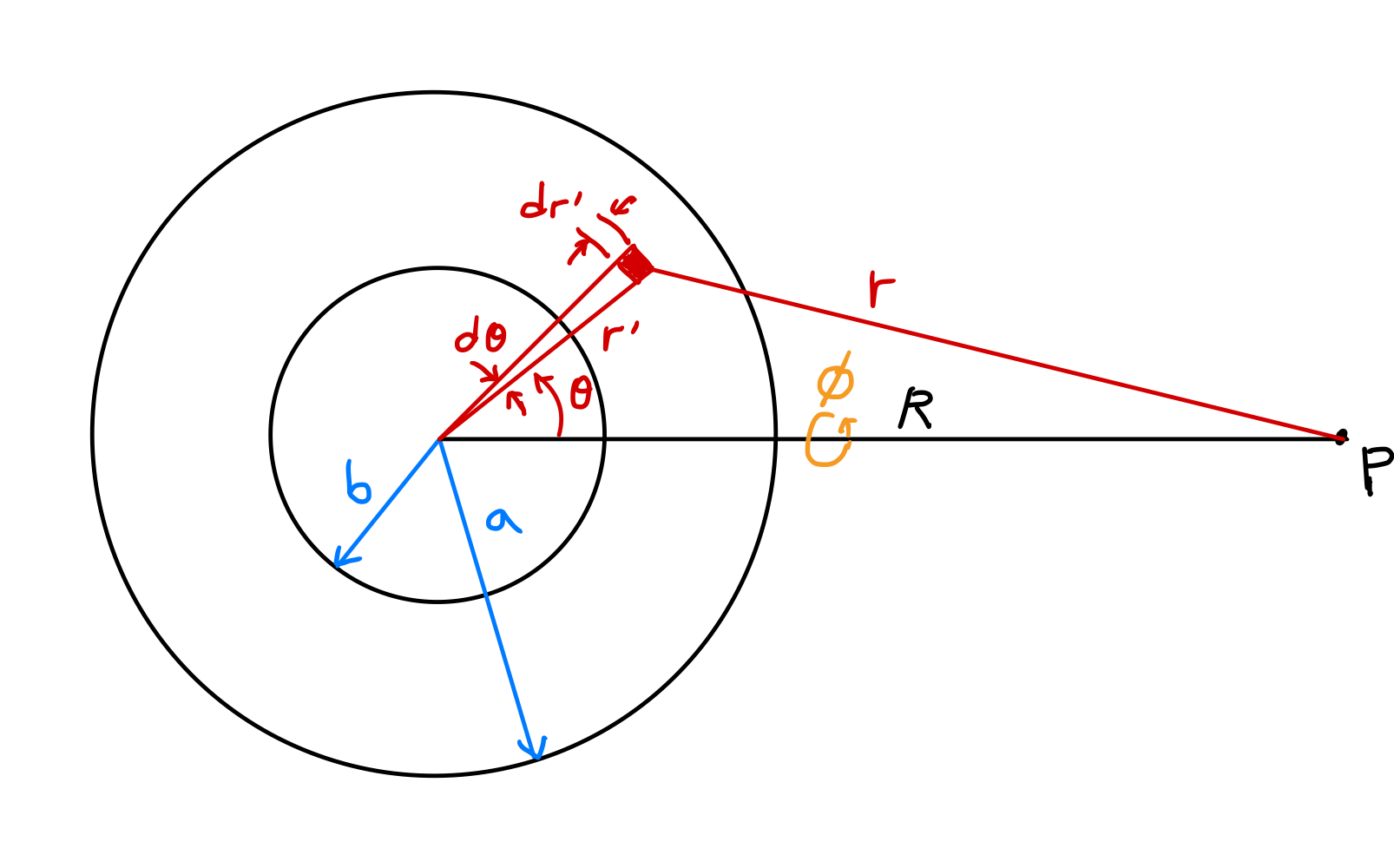
In the figure above, let’s calculate the potential at point $P$ at distance $R$ from the center. Assuming uniform mass distribution in the shell, $\rho(r^\prime)=\rho$, and due to symmetry about the azimuthal angle $\phi$ with respect to the line connecting the sphere’s center and point $P$:

\[\begin{align*} \Phi &= -G\int_V \frac{\rho(r^\prime)}{r}dv^\prime \\ &= -\rho G \int_0^{2\pi} \int_0^\pi \int_b^a \frac{1}{r}(dr^\prime)(r^\prime d\theta)(r^\prime \sin\theta\, d\phi) \\ &= -\rho G \int_0^{2\pi} d\phi \int_b^a {r^\prime}^2 dr^\prime \int_0^\pi \frac{\sin\theta}{r}d\theta \\ &= -2\pi\rho G \int_b^a {r^\prime}^2 dr^\prime \int_0^\pi \frac{\sin\theta}{r}d\theta. \label{eqn:spherical_shell_1}\tag{13} \end{align*}\]

By the law of cosines:

\[r^2 = {r^\prime}^2 + R^2 - 2r^\prime R \cos\theta \label{eqn:law_of_cosines}\tag{14}\]

Since $R$ is constant, differentiating this equation with respect to $r^\prime$:

\[2rdr = 2r^\prime R \sin\theta d\theta\] \[\frac{\sin\theta}{r}d\theta = \frac{dr}{r^\prime R} \tag{15}\]

Substituting this into equation ($\ref{eqn:spherical_shell_1}$):

\[\Phi = -\frac{2\pi\rho G}{R} \int_b^a r^\prime dr^\prime \int_{r_\mathrm{min}}^{r_\mathrm{max}} dr. \label{eqn:spherical_shell_2}\tag{16}\]

Here, $r_\mathrm{max}$ and $r_\mathrm{min}$ are determined by the position of point $P$.

When $R>a$

\(\begin{align*} \Phi(R>a) &= -\frac{2\pi\rho G}{R} \int_b^a r^\prime dr^\prime \int_{R-r^\prime}^{R+r^\prime} dr \\ &= - \frac{4\pi\rho G}{R} \int_b^a {r^\prime}^2 dr^\prime \\ &= - \frac{4}{3}\frac{\pi\rho G}{R}(a^3 - b^3). \label{eqn:spherical_shell_outside_1}\tag{17} \end{align*}\)

The mass $M$ of the spherical shell is:

\[M = \frac{4}{3}\pi\rho(a^3 - b^3) \label{eqn:mass_of_shell}\tag{18}\]

Therefore, the potential is:

\[\boxed{\Phi(R>a) = -\frac{GM}{R}} \label{eqn:spherical_shell_outside_2}\tag{19}\]

Comparing the gravitational potential due to a point mass of mass $M$ in equation ($\ref{eqn:g_potential}$) with the result just obtained ($\ref{eqn:spherical_shell_outside_2}$), we see they are identical. This means that when calculating the gravitational potential at any external point due to a spherically symmetric mass distribution, we can assume all mass is concentrated at the center. Most spherical celestial bodies of a certain size or larger, such as Earth or the Moon, fall into this category, as they can be considered as countless spherical shells with the same center but different diameters nested like Matryoshka dolls. This provides the justification for assuming celestial bodies like Earth or the Moon as point masses without size in calculations mentioned at the beginning of this post.

When $R<b$

\(\begin{align*} \Phi(R<b) &= -\frac{2\pi\rho G}{R} \int_b^a r^\prime dr^\prime \int_{r^\prime - R}^{r^\prime + R}dr \\ &= -4\pi\rho G \int_b^a r^\prime dr^\prime \\ &= -2\pi\rho G(a^2 - b^2). \label{eqn:spherical_shell_inside}\tag{20} \end{align*}\)

Inside a spherically symmetric mass shell, the gravitational potential is constant regardless of position, and the gravitational force is $0$.

This is also a major reason why the “Hollow Earth theory,” one of the representative pseudosciences, is nonsense. If Earth were a spherical shell with a hollow interior as claimed by the Hollow Earth theory, no gravitational force would act on any object inside that cavity. Considering Earth’s mass and volume, such a hollow cannot exist, and even if it did, life forms there would not live with the inner surface of the spherical shell as ground, but would float in a weightless state like in a space station.
Microorganisms may live several kilometers deep underground, but at least not in the form claimed by the Hollow Earth theory. I also really enjoy Jules Verne’s novel “Journey to the Center of the Earth” and the movie “Journey to the Center of the Earth,” but we should enjoy fiction as fiction and not seriously believe it.

When $b<R<a$

\(\begin{align*} \Phi(b<R<a) &= -\frac{4\pi\rho G}{3R}(R^3 - b^3) - 2\pi\rho G(a^2 - R^2) \\ &= -4\pi\rho G \left( \frac{a^2}{2} - \frac{b^3}{3R} - \frac{R^2}{6} \right) \label{eqn:within_spherical_shell}\tag{21} \end{align*}\)

Results

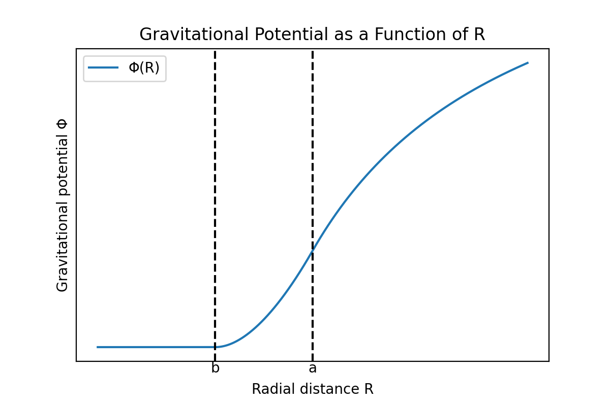
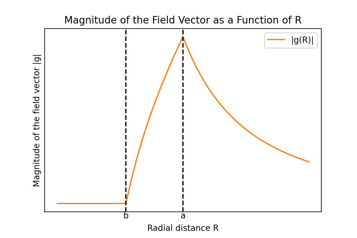
The gravitational potential $\Phi$ in the three regions obtained above, and the corresponding magnitude of the gravitational field vector $|\mathbf{g}|$ as functions of distance $R$, are shown graphically as follows:

• Python visualization code: yunseo-kim/physics-visualizations repository
• License: See here

We can see that both the gravitational potential and the magnitude of the gravitational field vector are continuous. If the gravitational potential were discontinuous at any point, the gradient of the potential at that point, i.e., the magnitude of gravity, would become infinite, which is not physically reasonable, so the potential function must be continuous at all points. However, the derivative of the gravitational field vector is discontinuous at the inner and outer surfaces of the shell.

Example: Galactic Rotation Curves

According to astronomical observations, in many spiral galaxies that rotate about their centers, such as the Milky Way and Andromeda Galaxy, most of the observable mass is concentrated near the center. However, the orbital velocities of masses in these spiral galaxies greatly disagree with theoretically predicted values based on the observable mass distribution, as can be seen in the following graph, and remain nearly constant beyond a certain distance.

Image source

• Author: Wikipedia user PhilHibbs
• License: Public Domain

Rotation curve of spiral galaxy M33 (Triangulum Galaxy)

• Author: Wikimedia user Mario De Leo
• License: CC BY-SA 4.0

Let’s predict the orbital velocity as a function of distance when the galaxy’s mass is concentrated at the center, confirm that this prediction does not match the observational results, and show that the mass $M(R)$ distributed within distance $R$ from the galactic center must be proportional to $R$ to explain the observations.

First, if the galactic mass $M$ is concentrated at the center, the orbital velocity at distance $R$ is:

\[\frac{GMm}{R^2} = \frac{mv^2}{R}\] \[v = \sqrt{\frac{GM}{R}} \propto \frac{1}{\sqrt{R}}.\]

In this case, an orbital velocity decreasing as $1/\sqrt{R}$ is predicted, as shown by the dotted lines in the two graphs above. However, according to observational results, the orbital velocity $v$ is nearly constant regardless of distance $R$, so the prediction and observations do not match. These observational results can only be explained if $M(R)\propto R$.

Setting $M(R) = kR$ using proportionality constant $k$:

\[v = \sqrt{\frac{GM(R)}{R}} = \sqrt{Gk}\ \text{(constant)}.\]

From this, astrophysicists conclude that many galaxies must contain undiscovered “dark matter,” and this dark matter must account for more than 90% of the universe’s mass. However, the identity of dark matter has not yet been clearly revealed, and while not mainstream theory, attempts like Modified Newtonian Dynamics (MOND) exist to explain observational results without assuming the existence of dark matter. Today, these research fields are at the forefront of astrophysics.